Understanding the Observability Stack in AKS

In the previous post on AKS Identity and Access Control, we covered authentication and authorisation, Workload Identity, secrets management, and Zero Trust principles.

Your cluster is now secured! But a cluster you cannot see into is a cluster you cannot operate. In production, pods crash, nodes exhaust resources, latency spikes, and deployments fail silently. Without observability, you are reacting to outages instead of preventing them.

This post covers the full observability stack for AKS: the layers you need to monitor, the Log Analytics tables and tiers to use, the new OpenTelemetry-native ingestion path, and how AKS Automatic changes the defaults.

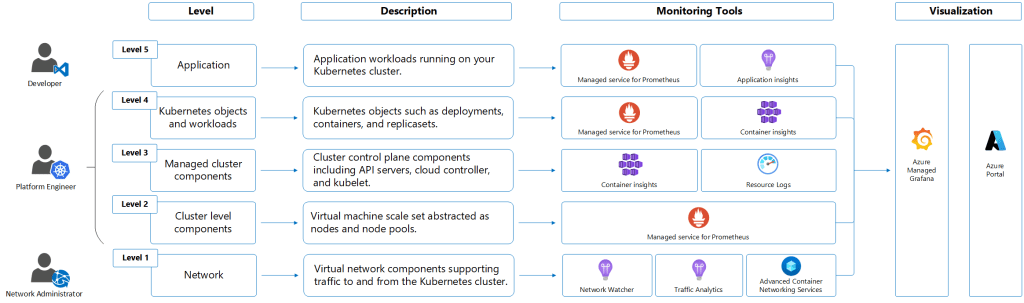
Observability Layers in AKS

I’ve used my “Onions have Layers, Kubernetes has Layers” meme previously, but the concepts of layers in AKS and Kubernetes in general becomes more visible when it comes to monitoring because there is no “single pane of glass, one-size fits all solution”. AKS monitoring operates across multiple distinct layers, and each layer requires a different set of tools.

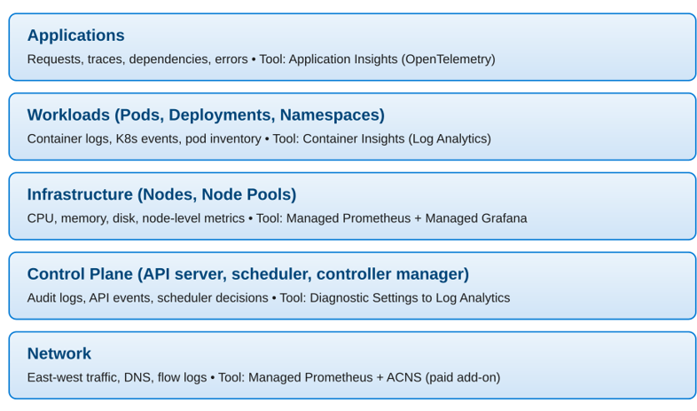
Each layer feeds into the others. A node running out of memory (Infrastructure layer) causes pod evictions (Workloads layer), which increase error rates (Applications layer). Full-stack observability means you can trace a user-facing incident from symptom to root cause across all layers.

Control Plane Logs

AKS is a managed service, so you do not have direct access to control plane nodes. Control plane activity is exposed as resource logs in Azure Monitor and enabling them is one of the first things you should do with any production cluster.

They are not collected by default. You must create a Diagnostic Setting on the cluster. Use resource-specific mode when creating the Diagnostic Setting. This routes logs to dedicated tables (AKSAudit, AKSAuditAdmin, AKSControlPlane) instead of the generic AzureDiagnostics table. Only resource-specific mode supports the Basic logs tier, which matters for cost control.

Category	What It Contains	When to Enable
kube-apiserver	All API server requests and responses	When troubleshooting API-level issues
kube-audit	Full audit log: all API calls including GET and LIST	When you need a complete interaction trail (high volume, high cost)
kube-audit-admin	Audit log scoped to write operations only (create, update, delete)	Recommended for most production clusters — lower cost than kube-audit
kube-controller-manager	Reconciliation loops and controller activity	Troubleshooting deployment and resource issues
kube-scheduler	Pod scheduling decisions	Diagnosing pending pods and scheduling failures
cluster-autoscaler	Scale-out and scale-in events	Always recommended on clusters using autoscaling
guard	Entra ID and Azure RBAC authentication audit events	Always recommended when using Entra ID integration

Infrastructure and Workload Metrics: Managed Prometheus and Grafana

Platform metrics (basic CPU, memory, and pod counts surfaced in the Azure portal) give you a starting point, but they are not enough for production operations. For real observability at the infrastructure and workload level, you need Azure Monitor Managed Service for Prometheus paired with Azure Managed Grafana.

Azure Monitor Managed Service for Prometheus

Managed Prometheus is a fully managed, Prometheus-compatible metrics service backed by an Azure Monitor workspace. It scrapes metrics from your AKS cluster using a containerized Azure Monitor agent deployed as a DaemonSet. There is no Prometheus server to deploy, scale, or maintain.

Key capabilities include:

Write your own queries or use community dashboards
Pre-configured recording rules and alert rules for Kubernetes deployed automatically
Metrics retention for up to 18 months
Native integration with Azure Managed Grafana for visualisation
Enabled with –enable-azure-monitor-metrics at cluster creation or update

Azure Managed Grafana

Azure Managed Grafana is a fully managed Grafana instance that connects directly to your Azure Monitor workspace as a data source. It comes pre-loaded with community Kubernetes dashboards covering node health, pod resource consumption, API server performance, and more.

You can link a Grafana workspace to your cluster at the same time you enable Prometheus metrics. A single Azure Managed Grafana instance can serve as a single pane of glass across multiple AKS clusters, all pointing at the same Azure Monitor workspace.

Container Insights: Logs, Events, and Workload Visibility

Container Insights is a feature of Azure Monitor that collects container logs, Kubernetes events, and workload inventory from your AKS cluster and stores them in a Log Analytics workspace. It is the primary tool for understanding what is happening inside your pods and namespaces.

Container Insights and Managed Prometheus work together using the same containerized Azure Monitor agent. Prometheus handles metrics, Container Insights handles logs and events.

What Container Insights Collects

Container logs: stdout and stderr from all containers, stored in ContainerLogV2 (the recommended schema)
Kubernetes events: pod restarts, scheduling failures, image pull errors, OOM kills
Pod and node inventory: workload state, resource requests and limits, namespace breakdown
Performance data: CPU and memory utilisation at node and container level

Data collection can be customised using Azure Monitor Data Collection Rules (DCRs) to control costs . You can configure collection intervals, exclude namespaces, and select specific tables to reduce ingestion volume.

Important ContainerLogV2 is the recommended log schema for new clusters. It provides structured fields including pod name, namespace, and container name, making queries significantly easier than the legacy ContainerLog schema.

Application-Level Observability: Application Insights

Infrastructure and workload observability tells you that a pod is crashing or a node is under pressure. Application Insights tells you why users are seeing errors — which requests are failing, where latency is concentrated, and how services are calling each other.

Application Insights is an application performance monitoring (APM) feature of Azure Monitor. For AKS workloads, there are three instrumentation approaches:

Code-Based Instrumentation with OpenTelemetry

The standard approach is to add the Azure Monitor OpenTelemetry Distro to your application code. This collects requests, dependencies, exceptions, traces, and custom metrics, sending them to an Application Insights resource.

This gives you the Application Map along with Live Metrics for real-time visibility into production traffic.

Automatic Instrumentation (Preview)

When automatic instrumentation is enabled, the Azure Monitor OpenTelemetry Distro is injected into application pods automatically with no code changes required. Instrumentation can be applied on all namespaces or per-deployment.

Native OTLP Ingestion into Azure Monitor (Preview)

This is the recent announcement, and it is a significant shift. Azure Monitor now supports native ingestion of OpenTelemetry Protocol (OTLP) signals directly.

This annoucement is meaningful for a number of reasons., but the main one is that its vendor-neutral, so applications can use the standard open-source OpenTelemetry SDK and OTLP exporter with no Azure-specific code changes or configuration required.

Network Observability

Networking is often the last layer to get proper observability, yet it is frequently the source of hard-to-diagnose issues.

When Managed Prometheus is enabled on Kubernetes 1.29 or later, basic node-level network metrics are collected by default via the Retina-based scraper, covering traffic volume and error rates.

For deeper visibility, including pod-level metrics, DNS tracking, and full flow logs, Container Network Observability (part of Advanced Container Networking Services) provides eBPF-based telemetry and writes results to ContainerNetworkLogs and RetinaNetworkFlowLogs. ACNS is a paid add-on.

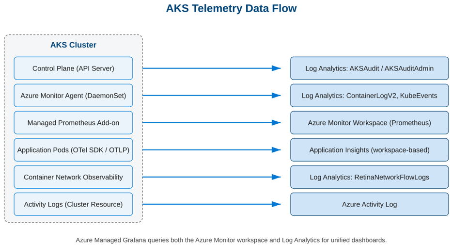
Telemetry Data Flow

And breathe! With so many tools collecting from so many sources, it helps to see the full picture:

Log Analytics Tables and Tiers

Anyone who follows me on LinkedIn (sneaky link for those who don’t!) knows that I talk a lot about FinOps and that Log Analytics is the target of a lot of my angst when it comes to Cost Management. For the sake of repeating myself, Log Analytics offers three table tiers, and the right choice for each AKS table can reduce your monitoring bill significantly.

Tier	Ingestion Cost	Best For
Analytics	Standard	Frequently queried data, alerting, dashboards
Basic	Significant discount	Verbose logs accessed occasionally
Auxiliary	Lowest cost	Long-term retention, rarely queried

When you send data to Log Analytics from any Azure resource, all tables default to the “Analytics” tier. For AKS which is a high procesing system with multiple layers which can generate a high volume of logs, you need to think about how these will be stored in Log Analytics. Below is a sample of how this should look:

Table	Source	Tier	Why
AKSAudit	kube-audit	✅ Basic	Very high volume. Compliance and investigation, not real-time alerting
AKSAuditAdmin	kube-audit-admin	Analytics	Write operations only. Often used for alerting and security
AKSControlPlane	Other control plane logs	Analytics	Operational data used for troubleshooting and alerting
ContainerLogV2	Container Insights	✅ Basic	Container stdout/stderr. Very high volume. Microsoft recommends Basic
KubeEvents	Container Insights	Analytics	Pod restarts, OOM kills, scheduling failures. Critical for alerting
KubePodInventory	Container Insights	Analytics	Powers Container Insights UI. Must be Analytics
RetinaNetworkFlowLogs	Container Network Observability	✅ Basic	Switch from Analytics default for cost savings

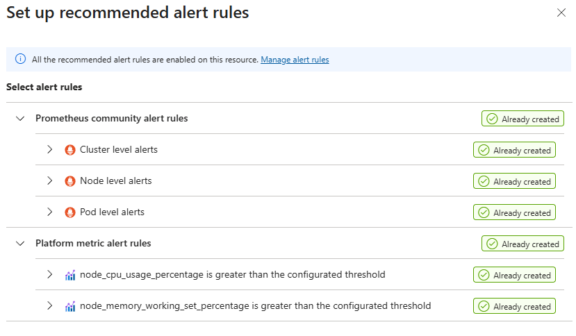
Alerting and Recommended Alert Rules

Collecting data is only useful if you act on it. Azure Monitor provides a set of recommended Prometheus-based alert rules for AKS that you can enable with a single action in the portal. These cover the most important cluster health signals:

Node CPU and memory pressure
Pod restart rates and CrashLoopBackOff detection
Pending pods – pods that cannot be scheduled
Job failures
Container OOM (out of memory) kills
PersistentVolume capacity

These rules are backed by Prometheus metrics and stored in your Azure Monitor workspace.

AKS Automatic: How Observability Defaults Change

Everything covered so far assumes an AKS Standard cluster, where observability is opt-in. On a fresh Standard cluster, nothing is enabled by default. AKS Automatic is different. It is a more opinionated, fully managed cluster experience where observability comes preconfigured.

Component	AKS Standard	AKS Automatic
Managed Prometheus	❌ Optional	✅ Default at creation
Container Insights	❌ Optional	✅ Default at creation
ACNS Container Network Observability	❌ Optional (paid)	✅ Default (portal creation)
Managed Grafana workspace	❌ Optional	❌ Optional
Diagnostic Settings (control plane)	❌ Optional	❌ Optional
Recommended Prometheus alert rules	❌ Optional	❌ Optional

The TLDR: AKS Automatic gives you a much stronger observability baseline from minute one. But control plane Diagnostic Settings (kube-audit-admin, guard) are still not on by default, and the Log Analytics tier configuration is still your responsibility.

Aligning with the Azure Well-Architected Framework

Operational Excellence: Full-stack observability means faster to detect and faster to resolve. Prebuilt dashboards (remember, someone needs to be looking at them!) and alert rules (remember, someone needs to act on them and not just have an Outlook rule that puts them in a folder where they are ignored) reduce the time to configure baseline monitoring.
Reliability: Alerting on node pressure, pending pods, and OOM events allows teams to respond before workloads are disrupted. Kubernetes event collection surfaces early warning signals.
Security: kube-audit-admin and guard logs provide an audit trail for all API write operations and authentication events, supporting compliance and incident investigation.
Cost Optimisation: Data Collection Rules allow you to control ingestion volume. Using kube-audit-admin instead of kube-audit, configuring collection intervals, and filtering namespaces can significantly reduce Log Analytics and Prometheus costs.

Conclusion

At this stage in our AKS journey we have designed the AKS architecture, networking, control plane connectivity, traffic flow, identity and access control, and now observability. The cluster is secure, well-networked, and visible.

In the next post we turn to scaling and node management — how AKS handles demand changes, how to design node pools for production workloads, and how the Cluster Autoscaler and KEDA work together to keep costs under control while maintaining availability.

See you on the next post – while you’re waiting for that you can check out the rest of the posts in the series here.

Monitoring with Grafana and InfluxDB using Docker Containers — Part 4: Install and Use Telegraf with PowerShell, send data to InfluxDB, and get the Dashboard working!

This post originally appeared on Medium on May 14th 2021

Welcome to Part 4 and the final part of my series on setting up Monitoring for your Infrastructure using Grafana and InfluxDB.

This image has an empty alt attribute; its file name is 0*gj-SHaUJ-slesruN

Last time, we set up InfluxDB as our Datasource for the data and metrics we’re going to use in Grafana. We also download the JSON for our Dashboard from the Grafana Dashboards Site and import this into Grafana instance. This finished off the groundwork of getting our Monitoring System built and ready for use.

In the final part, I’ll show you how to install the Telegraf Data collector agent on our WSUS Server. I’ll then configure the telgraf.conf file to query a PowerShell script, which will in turn send all collected metrics back to our InfluxDB instance. Finally, I’ll show you how to get the data from InfluxDB to display in our Dashboard.

Telegraf Install and Configuration on Windows

Telegraf is a plugin-driven server agent for collecting and sending metrics and events from databases, systems, and IoT sensors. It can be downloaded directly from the InfluxData website, and comes in version for all OS’s (OS X, Ubuntu/Debian, RHEL/CentOS, Windows). There is also a Docker image available for each version!

To download for Windows, we use the following command in Powershell:

wget https://dl.influxdata.com/telegraf/releases/telegraf-1.18.2_windows_amd64.zip -UseBasicParsing -OutFile telegraf-1.18.2_windows_amd64.zip

This downloads the file locally, you then use this command to extract the archive to the default destination:

Expand-Archive .\telegraf-1.18.2_windows_amd64.zip -DestinationPath 'C:\Program Files\InfluxData\telegraf\'

Once the archive gets extracted, we have 2 files in the folder: telegraf.exe, and telegraf.conf:

Telegraf.exe is the Data Collector Service file and is natively supported running as a Windows Service. To install the service, run the following command from PowerShell:

C:\"Program Files"\InfluxData\Telegraf\Telegraf-1.18.2\telegraf.exe --service install

This will install the Telegraf Service, as shown here under services.msc:

Telegraf.conf is the parameter file, and telegraf.conf reads that to see what metrics it needs to collect and send to the specified destination. The download I did above contains a template telegraf.conf file which will return the recommended Windows system metrics.

To test that the telgraf is working, we’ll run this command from the directory where telegraf.exe is located:

.\telegraf.exe --config telegraf.conf --test

As we can see, this is running telgraf.exe and specifying telgraf.conf as its config file. This will return this output:

This shows that telegraf can collect data from the system and is working correctly. Lets get it set up now to point at our InfluxDB. To do this, we open our telgraf.conf file and go to the [[outputs.influxdb]] section where we add this info:

[[outputs.influxdb]]

urls = ["http://10.210.239.186:8086"] 
  database = "telegraf" 
  precision = "s"
  timeout = "10s"

This is specifying the url/port and database where we want to send the data to. This is the basic setup for telegraf.exe, next up I’ll get it working with our PowerShell script so we can send our WSUS Metrics into InfluxDB.

Using Telegraf with PowerShell

As a prerequisite, we’ll need to install the PoshWSUS Module on our WSUS Server, which can be downloaded from here.

Once this is installed, we can download our WSUS PowerShell script. The link to the script can be found here. If we look at the script, its going to do the following:

Get a count of all machines per OS Version
Get the number of updates pending for the WSUS Server
Get a count of machines that need updates, have failed updates, or need a reboot
Return all of the above data to the telegraf data collector agent, which will send it to the InfluxDB.

Before doing any integration with Telegraf, modify the script to your needs using PowerShell ISE (on line 26, you need to specify the FQDN of your own WSUS Server), and then run the script to make sure it returns the data you expect. The result will look something like this

This tells us that the script works. Now we can integrate the script into our telegraf.conf file. Underneath the “Inputs” section of the file, add the following lines:

####################################################################
#                        INPUTS                                    #
####################################################################

[[inputs.exec]]
  commands = ["powershell C:/temp/wsus-stats.ps1"]
  name_override = "wsusstats"
  interval = "300s"
  timeout = "300s"
  data_format = "influx"

This is telling our telegraf.exe service to call PowerShell to run our script at an interval of 300 seconds, and return the data in “influx” format.

Now once we save the changes, we can test our telegraf.conf file again to see if it returns the data from the PowerShell script as well as the default Windows metrics. Again, we run:

.\telegraf.exe --config telegraf.conf --test

And this time, we should see the WSUS results as well as the Windows Metrics:

And we do! Great, and at this point, we can now change our Telegraf Service that we installed earlier to “Running” by running this command:

net start telegraf

Now that we have this done, lets get back into Grafana and see if we can get some of this data to show in the Dashboard!

Configuring Dashboards

In the last post, we imported our blank dashboard using our json file.

Now that we have our Telegraf Agent and PowerShell script working and sending data back to InfluxDB, we can now start configuring the panels on our dashboard to show some data.

For each of the panels on our dashboard, clicking on the title at the top reveals a dropdown list of actions.

As you can see, there are a number of actions you can take (including removing a panel if you don’t need it), however we’re going to click on “Edit”. This brings us into a view where we get access to modify the properties of the Query, and also can modify some Dashboard settings including the Title and color’s to show based on the data that is being returned:

The most important thing for use in this screen is the query

As you can see, in the “FROM” portion of the query, you can change the values for “host” to match the hostname of your server. Also, from the “SELECT” portion, you can change the field() to match the data that you need to have represented on your panel. If we take a look at this field and click, it brings us a dropdown:

Remember where these values came from? These are the values that we defined in our PowerShell script above. When we select the value we want to display, we click “Apply” at the top right of the screen to save the value and return to the Main Dashboard:

And there’s our value displayed! Lets take a look at one of the default Windows OS Metrics as well, such as CPU Usage. For this panel, you just need to select the “host” where you want the data to be displayed from:

And as we can see, its gets displayed:

There’s a bit of work to do in order to get the dashboard to display all of the values on each panel, but eventually you’ll end up with something looking like this:

As you can see, the data on the graph panels is timed (as this is a time series database), and you can adjust the times shown on the screen by using the time period selector at the top right of the Dashboard:

The final thing I’ll show you is if you have multiple Dashboards that you are looking to display on a screen, Grafana can do this by using the “Playlists” option under Dashboards.

You can also create Alerts to go to multiple sources such as Email, Teams Discord, Slack, Hangouts, PagerDuty or a webhook.

Conclusion

As you have seen over this post, Grafana is a powerful and useful tool for visualizing data. The reason for using this is conjunction with InfluxDB and Telegraf is that it had native support for Windows which was what we needed to monitor.

You can use multiple data sources (eg Prometheus, Zabbix) within the same Grafana instance depending on what data you want to visualize and display. The Grafana Dashboards site has thousands of community and official Dashboards for multiple systems such as AWS, Azure, Kubernetes etc.

While Grafana is a wonderful tool, its should be used as part of your monitoring infrastructure. Dashboards provide a great “birds-eye” view of the status of your Infrastructure, but you should use these in conjunction with other tools and processes, such as using alerts to generate tickets or self-healing alerts based on thresholds.

Thanks again for reading, I hope you have enjoyed the series and I’ll see you on the next one!

Monitoring with Grafana and InfluxDB using Docker Containers — Part 3: Datasource Configuration and Dashboard Installation

This post originally appeared on Medium on May 5th 2021

Welcome to Part 3 of my series on setting up Monitoring for your Infrastructure using Grafana and InfluxDB.

Last time, we downloaded our Docker Images for Grafana and InfluxDB, created persistent storage for them to persist our data, and also configured our initial Influx Database that will hold all of our Data.

In Part 3, we’re going to set up InfluxDB as our Datasource for the data and metrics we’re going to use in Grafana. We’ll also download the JSON for our Dashboard from the Grafana Dashboards Site and import this into Grafana instance. This will finish off the groundwork of getting our Monitoring System built and ready for use.

Configure your Data Source

Now we have our InfluxDB set up, we’re ready to configure it as a Data source in Grafana. So we log on to the Grafana console. Click the “Configuration” button (looks like a cog wheel) on the left hand panel, and select “Data Sources”

This is the main config screen for the Grafana Instance. Click on “Add data source”

Search for “influxdb”. Click on this and it will add it as a Data Source:

We are now in the screen for configuring our InfluxDB. We configure the following options:
Query Language — InfluxQL. (there is an option for “Flux”, however this is only used by InfluxDB versions newer than 1.8)
URL — this is the Address of our InfluxDB container instance. Don’t forget to specify the port as 8086.
Access — This will always be Server
Auth — No options needed here

Finally, we fill in our InfluxDB details:
Database — this is the name that we defined when setting up the database, in our case telegraf
User — this is our “johnboy” user
Password — This is the password
Click on “Save & Test”. This should give you a message saying that the Data source is working — this means you have a successful connection between Grafana and InfluxDB.

Great, so now we have a working connection between Grafana and InfluxDB

Dashboards

We now have our Grafana instance and our InfluxDB ready. So now we need to get some data into our InfluxDB and use this in some Dashboards. The Grafana website (https://grafana.com/grafana/dashboards) has hundreds of official and community build dashboards.

As a reminder, the challenge here is to visualize WSUS … yes, I know WSUS. As in Windows Server Update Services. Sounds pretty boring doesn’t it? It’s not really though — the problem is that unless WSUS is integrated with the likes of SCCM, SCOM or some other 3rd party tools (all of which will incur Licensing Costs), it doesn’t really have a good way of reporting and visualizing its content in a Dashboard.

I’ll go to the Grafana Dashboards page and search for WSUS. We can also search by Data Source.

When we click into the first option, we can see that we can “Download JSON”

Once this is downloaded, lets go back to Grafana. Open Dashboards, and click “Import”:

Then we can click “Upload JSON File” and upload our downloaded json. We can also import directly from the Grafana website using the Dashboard ID, or else paste the JSON directly in:

Once the JSON is uploaded, you then get the screen below where you can rename the Dashboard, and specify what Data Source to use. Once this is done, click “Import”:

And now we have a Dashboard. But there’s no data! That’s the next step, we need to configure our WSUS Server to send data back to the InfluxDB.

Next time …..

Thanks again for reading! Next time will be the final part of our series, where we’ll install the Telegraf agent on our WSUS Server, use it to run a PowerShell script which will send data to our InfluxDB, and finally bring the data from InfluxDB into our Grafana Dashboard.

Hope you enjoyed this post, until next time!!

Monitoring with Grafana and InfluxDB using Docker Containers — Part 2: Docker Image Pull and Setup

This post originally appeared on Medium on April 19th 2021

Welcome to Part 2 of my series on setting up Monitoring for your Infrastructure using Grafana and InfluxDB.

Last week as well as the series Introduction, we started our Monitoring build with Part 1, which was creating our Ubuntu Server to serve as a host for our Docker Images. Onwards we now go to Part 2, where the fun really starts and we pull our images for Grafana and InfluxDB from Docker Hub, create persistent storage and get them running.

Firstly, lets get Grafana running!

We’re going to start by going to the official Grafana Documentation (link here) which tells us that we need to create a persistent storage volume for our container. If we don’t do this, all of our data will be lost every time the container shuts down. So we run sudo docker volume create grafana-storage:

That’s created, but where is it located? Run this command to find out: sudo find / -type d -name “grafana-storage

This tells us where the file location is (in this case, the location as we can see above is:

var/snap/docker/common/var-lib-docker/volumes/grafana-storage

Now, we need to download the Grafana image from the docker hub. Run sudo docker search grafana to search for a list of Grafana images:

As we can see, there are a number of images available but we want to use the official one at the top of the list. So we run sudo docker pull grafana/grafana to pull the image:

This will take a few seconds to pull down. We run the sudo docker images command to confirm the image has downloaded:

Now the image is downloaded and we have our storage volume ready to persist our data. Its time to get our image running. Lets run this command:

sudo docker run -d -p 3000:3000 — name=grafana -v grafana-storage:var/snap/docker/common/var-lib-docker/volumes/grafana-storage grafana/grafana

Wow, that’s a mouthful ….. lets explain what the command is doing. We use “docker run -d” to start the container in the background. We then use the “-p 3000:3000” to make the container available on port 3000 via the IP Address of the Ubuntu Host. We then use “-v” to point at our persistent storage location that we created, and finally we use “grafana/grafana” to specify the image we want to use.
The IP of my Ubuntu Server is 10.210.239.186. Lets see if we can browse to 10.210.239.186:3000 …..

Well hello there beautiful ….. the default username/password is admin/admin, and you will be prompted to change this at first login to something more secure.

Now we need a Data Source!

Now that we have Grafana running, we need a Data Source to store the data that we are going to present via our Dashboard. There are many excellent data sources available, the question is which one to use. That can be answered by going to the Grafana Dashboards page, where you will find thousands of Official and Community built dashboards. By searching for the Dashboard you want to create, you’ll quickly see the compatible Data Source for your desired dashboard. So if you recall, we are trying to visualize WSUS Metrics, and if we search for WSUS, we find this:

As you can see, InfluxDB is the most commonly used, so we’re going to use that. But what is this “InfluxDB” that I speak of.
InfluxDB is a “time series database”. The good people over at InfluxDB explain it a lot better than I will, but in summary a time series database is optimized for time-stamped data that can be tracked, monitored and sampled over time.
I’m going to keep using docker for hosting all elements of our monitoring solution. Lets search for the InfluxDB image on the Docker Hub by running sudo docker search influx:

Again, I’m going to use the official one, so run the sudo docker pull influxdb:1.8 command to pull the image. Note that I’m pulling the InfluxDB image with tag 1.8. Versions after 1.8 use a new DB Model which is not yet widely used:

And to confirm, lets run sudo docker images:

At this point, I’m ready to run the image. But first, lets create another persistent storage area on the host for the InfluxDB image, just like I did for the Grafana one. So we run sudo docker volume create influx18-storage:

Again, lets run the command to find it and get the exact location:

And this is what we need for our command to launch the container:

sudo docker run -d -p 8086:8086 — name=influxdb -v influx18-storage:var/snap/docker/common/var-lib-docker/volumes/influx18-storage influxdb:1.8

We’re running InfluxDB on port 8086 as this is its default. So now, lets check our 2 containers are running by running sudo docker ps:

OK great, so we have our 2 containers running. Now, we need to interact with the InfluxDB Container to create our database. So we run sudo docker exec -it 99ce /bin/bash:

This gives us an interactive session (docker exec -it) with the container (we’ve used the container ID “99ce” from above to identify it) so we can configure it. Finally, we’ve asked for a bash session (/bin/bash) to run commands from. So now, lets create our database and set authentication. We run “influx” and setup our database and user authentication:

Next time….

Great! So now that’s done , we need to configure InfluxDB as a Data Source for Grafana. You’ll have to wait for Part 3 for that! Thanks again for reading, and hope to see you back next week where as well as setting up our Data Source connection, we’ll set up our Dashboard in Grafana ready to receive data from our WSUS Server!

Hope you enjoyed this post, until next time!!

Monitoring with Grafana and InfluxDB using Docker Containers — Introduction

This post originally appeared on Medium on April 12th 2021

Welcome to a series where I’ll show you how to set up Monitoring for your Infrastructure using Grafana and InfluxDB.

A little bit about Monitoring ….

Monitoring is one of the most important parts of any infrastructure setup, whether On-Premise, Hybrid or Cloud based. Not only can it help with outages, performance and security , its also used for help in design and scaling of your infrastructure.

Traditionally, monitoring systems comprise of 3 components:

An agent to collect data from a source (this source can be an Operating System, Database, Application, Website or a piece of Hardware)
A central database to store the data collected by all of the agents
A website or application to visualize the data into a readable format

In the example shown below, the components are:

Windows (Operating System, which is the Source)
Telegraf (Data Collection Agent)
InfluxDB (Time Series Database to store data sent by the Agent)
Grafana (System to visualize the data in the database)

The Challenge

I was given a challenge to provide visualization for Microsoft Windows Server Update Services (WSUS). Anyone who uses this console knows that it hasn’t changed all that much since it was originally released way back in 2005, and any of the built in reporting leaves a lot to be desired:

Ugh …. there has to be a better way to do this …. And there is!!!

How I’ll build it!

To make things more interesting, I’m going to run Grafana and InfluxDB using Docker containers running on an Ubuntu Docker Host VM. Then we’re going to monitor a Microsoft WSUS Server with Telegraf Agent installed!

During the series, I’ll be showing you how to build the system from scratch using these steps:

Click on each of the links to go to the post — I’ll update the links as each post is released

Next time ….

Click here to go to the first step in building our Monitoring system, building our Ubuntu Docker Host

Hope you enjoyed this post, until next time!!