Monitoring with Grafana and InfluxDB using Docker Containers — Part 4: Install and Use Telegraf with PowerShell, send data to InfluxDB, and get the Dashboard working!

This post originally appeared on Medium on May 14th 2021

Welcome to Part 4 and the final part of my series on setting up Monitoring for your Infrastructure using Grafana and InfluxDB.

This image has an empty alt attribute; its file name is 0*gj-SHaUJ-slesruN

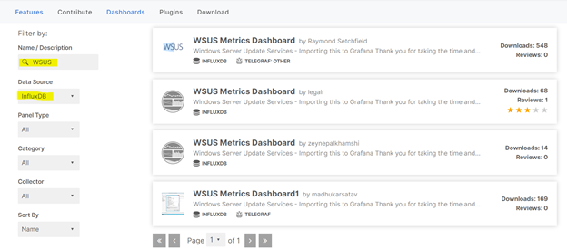
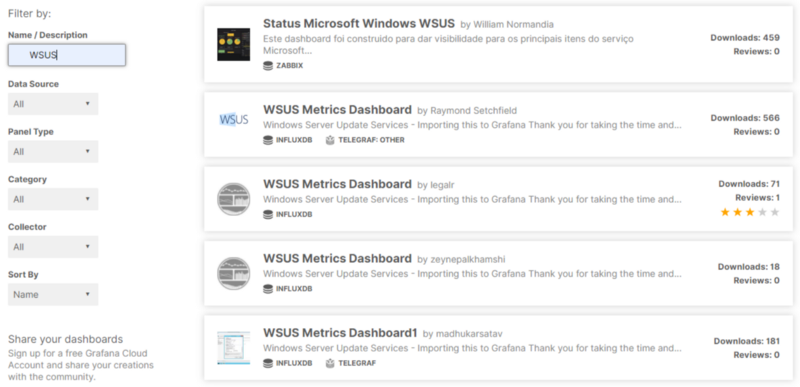
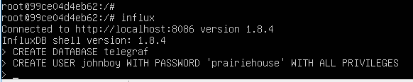
Last time, we set up InfluxDB as our Datasource for the data and metrics we’re going to use in Grafana. We also download the JSON for our Dashboard from the Grafana Dashboards Site and import this into Grafana instance. This finished off the groundwork of getting our Monitoring System built and ready for use.

In the final part, I’ll show you how to install the Telegraf Data collector agent on our WSUS Server. I’ll then configure the telgraf.conf file to query a PowerShell script, which will in turn send all collected metrics back to our InfluxDB instance. Finally, I’ll show you how to get the data from InfluxDB to display in our Dashboard.

Telegraf Install and Configuration on Windows

Telegraf is a plugin-driven server agent for collecting and sending metrics and events from databases, systems, and IoT sensors. It can be downloaded directly from the InfluxData website, and comes in version for all OS’s (OS X, Ubuntu/Debian, RHEL/CentOS, Windows). There is also a Docker image available for each version!

To download for Windows, we use the following command in Powershell:

wget https://dl.influxdata.com/telegraf/releases/telegraf-1.18.2_windows_amd64.zip -UseBasicParsing -OutFile telegraf-1.18.2_windows_amd64.zip

This downloads the file locally, you then use this command to extract the archive to the default destination:

Expand-Archive .\telegraf-1.18.2_windows_amd64.zip -DestinationPath 'C:\Program Files\InfluxData\telegraf\'

Once the archive gets extracted, we have 2 files in the folder: telegraf.exe, and telegraf.conf:

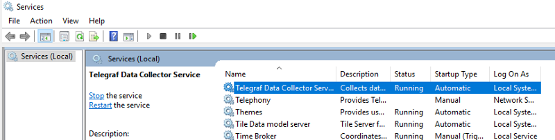
Telegraf.exe is the Data Collector Service file and is natively supported running as a Windows Service. To install the service, run the following command from PowerShell:

C:\"Program Files"\InfluxData\Telegraf\Telegraf-1.18.2\telegraf.exe --service install

This will install the Telegraf Service, as shown here under services.msc:

Telegraf.conf is the parameter file, and telegraf.conf reads that to see what metrics it needs to collect and send to the specified destination. The download I did above contains a template telegraf.conf file which will return the recommended Windows system metrics.

To test that the telgraf is working, we’ll run this command from the directory where telegraf.exe is located:

.\telegraf.exe --config telegraf.conf --test

As we can see, this is running telgraf.exe and specifying telgraf.conf as its config file. This will return this output:

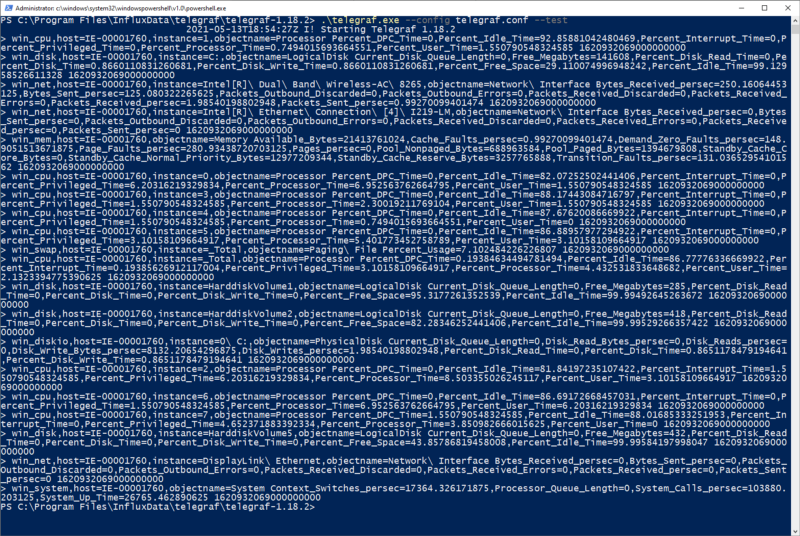
This shows that telegraf can collect data from the system and is working correctly. Lets get it set up now to point at our InfluxDB. To do this, we open our telgraf.conf file and go to the [[outputs.influxdb]] section where we add this info:

[[outputs.influxdb]]
urls = ["http://10.210.239.186:8086"] 
database = "telegraf"
precision = "s"
timeout = "10s"

This is specifying the url/port and database where we want to send the data to. This is the basic setup for telegraf.exe, next up I’ll get it working with our PowerShell script so we can send our WSUS Metrics into InfluxDB.

Using Telegraf with PowerShell

As a prerequisite, we’ll need to install the PoshWSUS Module on our WSUS Server, which can be downloaded from here.

Once this is installed, we can download our WSUS PowerShell script. The link to the script can be found here. If we look at the script, its going to do the following:

  • Get a count of all machines per OS Version
  • Get the number of updates pending for the WSUS Server
  • Get a count of machines that need updates, have failed updates, or need a reboot
  • Return all of the above data to the telegraf data collector agent, which will send it to the InfluxDB.

Before doing any integration with Telegraf, modify the script to your needs using PowerShell ISE (on line 26, you need to specify the FQDN of your own WSUS Server), and then run the script to make sure it returns the data you expect. The result will look something like this

This tells us that the script works. Now we can integrate the script into our telegraf.conf file. Underneath the “Inputs” section of the file, add the following lines:

####################################################################
# INPUTS #
####################################################################
[[inputs.exec]]
commands = ["powershell C:/temp/wsus-stats.ps1"]
name_override = "wsusstats"
interval = "300s"
timeout = "300s"
data_format = "influx"

This is telling our telegraf.exe service to call PowerShell to run our script at an interval of 300 seconds, and return the data in “influx” format.

Now once we save the changes, we can test our telegraf.conf file again to see if it returns the data from the PowerShell script as well as the default Windows metrics. Again, we run:

.\telegraf.exe --config telegraf.conf --test

And this time, we should see the WSUS results as well as the Windows Metrics:

And we do! Great, and at this point, we can now change our Telegraf Service that we installed earlier to “Running” by running this command:

net start telegraf

Now that we have this done, lets get back into Grafana and see if we can get some of this data to show in the Dashboard!

Configuring Dashboards

In the last post, we imported our blank dashboard using our json file.

Now that we have our Telegraf Agent and PowerShell script working and sending data back to InfluxDB, we can now start configuring the panels on our dashboard to show some data.

For each of the panels on our dashboard, clicking on the title at the top reveals a dropdown list of actions.

As you can see, there are a number of actions you can take (including removing a panel if you don’t need it), however we’re going to click on “Edit”. This brings us into a view where we get access to modify the properties of the Query, and also can modify some Dashboard settings including the Title and color’s to show based on the data that is being returned:

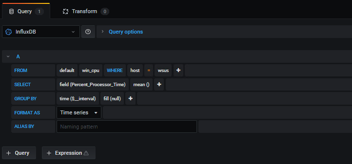
The most important thing for use in this screen is the query

As you can see, in the “FROM” portion of the query, you can change the values for “host” to match the hostname of your server. Also, from the “SELECT” portion, you can change the field() to match the data that you need to have represented on your panel. If we take a look at this field and click, it brings us a dropdown:

Remember where these values came from? These are the values that we defined in our PowerShell script above. When we select the value we want to display, we click “Apply” at the top right of the screen to save the value and return to the Main Dashboard:

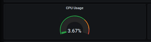
And there’s our value displayed! Lets take a look at one of the default Windows OS Metrics as well, such as CPU Usage. For this panel, you just need to select the “host” where you want the data to be displayed from:

And as we can see, its gets displayed:

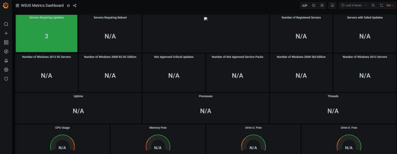
There’s a bit of work to do in order to get the dashboard to display all of the values on each panel, but eventually you’ll end up with something looking like this:

As you can see, the data on the graph panels is timed (as this is a time series database), and you can adjust the times shown on the screen by using the time period selector at the top right of the Dashboard:

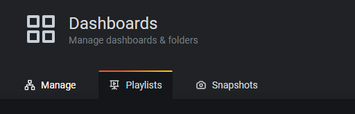
The final thing I’ll show you is if you have multiple Dashboards that you are looking to display on a screen, Grafana can do this by using the “Playlists” option under Dashboards.

You can also create Alerts to go to multiple sources such as Email, Teams Discord, Slack, Hangouts, PagerDuty or a webhook.

Conclusion

As you have seen over this post, Grafana is a powerful and useful tool for visualizing data. The reason for using this is conjunction with InfluxDB and Telegraf is that it had native support for Windows which was what we needed to monitor.

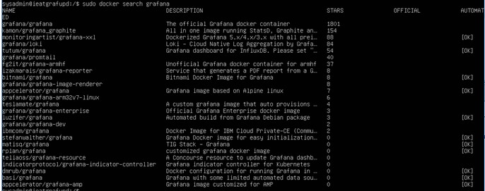
You can use multiple data sources (eg Prometheus, Zabbix) within the same Grafana instance depending on what data you want to visualize and display. The Grafana Dashboards site has thousands of community and official Dashboards for multiple systems such as AWS, Azure, Kubernetes etc.

While Grafana is a wonderful tool, its should be used as part of your monitoring infrastructure. Dashboards provide a great “birds-eye” view of the status of your Infrastructure, but you should use these in conjunction with other tools and processes, such as using alerts to generate tickets or self-healing alerts based on thresholds.

Thanks again for reading, I hope you have enjoyed the series and I’ll see you on the next one!

Monitoring with Grafana and InfluxDB using Docker Containers — Part 3: Datasource Configuration and Dashboard Installation

This post originally appeared on Medium on May 5th 2021

Welcome to Part 3 of my series on setting up Monitoring for your Infrastructure using Grafana and InfluxDB.

Last time, we downloaded our Docker Images for Grafana and InfluxDB, created persistent storage for them to persist our data, and also configured our initial Influx Database that will hold all of our Data.

In Part 3, we’re going to set up InfluxDB as our Datasource for the data and metrics we’re going to use in Grafana. We’ll also download the JSON for our Dashboard from the Grafana Dashboards Site and import this into Grafana instance. This will finish off the groundwork of getting our Monitoring System built and ready for use.

Configure your Data Source

  • Now we have our InfluxDB set up, we’re ready to configure it as a Data source in Grafana. So we log on to the Grafana console. Click the “Configuration” button (looks like a cog wheel) on the left hand panel, and select “Data Sources”
  • This is the main config screen for the Grafana Instance. Click on “Add data source”
  • Search for “influxdb”. Click on this and it will add it as a Data Source:
  • We are now in the screen for configuring our InfluxDB. We configure the following options:
  • Query Language — InfluxQL. (there is an option for “Flux”, however this is only used by InfluxDB versions newer than 1.8)
  • URL — this is the Address of our InfluxDB container instance. Don’t forget to specify the port as 8086.
  • Access — This will always be Server
  • Auth — No options needed here
  • Finally, we fill in our InfluxDB details:
  • Database — this is the name that we defined when setting up the database, in our case telegraf
  • User — this is our “johnboy” user
  • Password — This is the password
  • Click on “Save & Test”. This should give you a message saying that the Data source is working — this means you have a successful connection between Grafana and InfluxDB.
  • Great, so now we have a working connection between Grafana and InfluxDB

Dashboards

We now have our Grafana instance and our InfluxDB ready. So now we need to get some data into our InfluxDB and use this in some Dashboards. The Grafana website (https://grafana.com/grafana/dashboards) has hundreds of official and community build dashboards.

As a reminder, the challenge here is to visualize WSUS … yes, I know WSUS. As in Windows Server Update Services. Sounds pretty boring doesn’t it? It’s not really though — the problem is that unless WSUS is integrated with the likes of SCCM, SCOM or some other 3rd party tools (all of which will incur Licensing Costs), it doesn’t really have a good way of reporting and visualizing its content in a Dashboard.

  • I’ll go to the Grafana Dashboards page and search for WSUS. We can also search by Data Source.
  • When we click into the first option, we can see that we can “Download JSON”
  • Once this is downloaded, lets go back to Grafana. Open Dashboards, and click “Import”:
  • Then we can click “Upload JSON File” and upload our downloaded json. We can also import directly from the Grafana website using the Dashboard ID, or else paste the JSON directly in:
  • Once the JSON is uploaded, you then get the screen below where you can rename the Dashboard, and specify what Data Source to use. Once this is done, click “Import”:
  • And now we have a Dashboard. But there’s no data! That’s the next step, we need to configure our WSUS Server to send data back to the InfluxDB.

Next time …..

Thanks again for reading! Next time will be the final part of our series, where we’ll install the Telegraf agent on our WSUS Server, use it to run a PowerShell script which will send data to our InfluxDB, and finally bring the data from InfluxDB into our Grafana Dashboard.

Hope you enjoyed this post, until next time!!

Monitoring with Grafana and InfluxDB using Docker Containers — Part 2: Docker Image Pull and Setup

This post originally appeared on Medium on April 19th 2021

Welcome to Part 2 of my series on setting up Monitoring for your Infrastructure using Grafana and InfluxDB.

Last week as well as the series Introduction, we started our Monitoring build with Part 1, which was creating our Ubuntu Server to serve as a host for our Docker Images. Onwards we now go to Part 2, where the fun really starts and we pull our images for Grafana and InfluxDB from Docker Hub, create persistent storage and get them running.

Firstly, lets get Grafana running!

We’re going to start by going to the official Grafana Documentation (link here) which tells us that we need to create a persistent storage volume for our container. If we don’t do this, all of our data will be lost every time the container shuts down. So we run sudo docker volume create grafana-storage:

  • That’s created, but where is it located? Run this command to find out: sudo find / -type d -name “grafana-storage
  • This tells us where the file location is (in this case, the location as we can see above is:

var/snap/docker/common/var-lib-docker/volumes/grafana-storage

  • Now, we need to download the Grafana image from the docker hub. Run sudo docker search grafana to search for a list of Grafana images:
  • As we can see, there are a number of images available but we want to use the official one at the top of the list. So we run sudo docker pull grafana/grafana to pull the image:
  • This will take a few seconds to pull down. We run the sudo docker images command to confirm the image has downloaded:
  • Now the image is downloaded and we have our storage volume ready to persist our data. Its time to get our image running. Lets run this command:

sudo docker run -d -p 3000:3000 — name=grafana -v grafana-storage:var/snap/docker/common/var-lib-docker/volumes/grafana-storage grafana/grafana

  • Wow, that’s a mouthful ….. lets explain what the command is doing. We use “docker run -d” to start the container in the background. We then use the “-p 3000:3000” to make the container available on port 3000 via the IP Address of the Ubuntu Host. We then use “-v” to point at our persistent storage location that we created, and finally we use “grafana/grafana” to specify the image we want to use.
  • The IP of my Ubuntu Server is 10.210.239.186. Lets see if we can browse to 10.210.239.186:3000 …..
  • Well hello there beautiful ….. the default username/password is admin/admin, and you will be prompted to change this at first login to something more secure.

Now we need a Data Source!

  • Now that we have Grafana running, we need a Data Source to store the data that we are going to present via our Dashboard. There are many excellent data sources available, the question is which one to use. That can be answered by going to the Grafana Dashboards page, where you will find thousands of Official and Community built dashboards. By searching for the Dashboard you want to create, you’ll quickly see the compatible Data Source for your desired dashboard. So if you recall, we are trying to visualize WSUS Metrics, and if we search for WSUS, we find this:
  • As you can see, InfluxDB is the most commonly used, so we’re going to use that. But what is this “InfluxDB” that I speak of.
  • InfluxDB is a “time series database”. The good people over at InfluxDB explain it a lot better than I will, but in summary a time series database is optimized for time-stamped data that can be tracked, monitored and sampled over time.
  • I’m going to keep using docker for hosting all elements of our monitoring solution. Lets search for the InfluxDB image on the Docker Hub by running sudo docker search influx:
  • Again, I’m going to use the official one, so run the sudo docker pull influxdb:1.8 command to pull the image. Note that I’m pulling the InfluxDB image with tag 1.8. Versions after 1.8 use a new DB Model which is not yet widely used:
  • And to confirm, lets run sudo docker images:
  • At this point, I’m ready to run the image. But first, lets create another persistent storage area on the host for the InfluxDB image, just like I did for the Grafana one. So we run sudo docker volume create influx18-storage:
  • Again, lets run the command to find it and get the exact location:
  • And this is what we need for our command to launch the container:

sudo docker run -d -p 8086:8086 — name=influxdb -v influx18-storage:var/snap/docker/common/var-lib-docker/volumes/influx18-storage influxdb:1.8

  • We’re running InfluxDB on port 8086 as this is its default. So now, lets check our 2 containers are running by running sudo docker ps:
  • OK great, so we have our 2 containers running. Now, we need to interact with the InfluxDB Container to create our database. So we run sudo docker exec -it 99ce /bin/bash:
  • This gives us an interactive session (docker exec -it) with the container (we’ve used the container ID “99ce” from above to identify it) so we can configure it. Finally, we’ve asked for a bash session (/bin/bash) to run commands from. So now, lets create our database and set authentication. We run “influx” and setup our database and user authentication:

Next time….

Great! So now that’s done , we need to configure InfluxDB as a Data Source for Grafana. You’ll have to wait for Part 3 for that! Thanks again for reading, and hope to see you back next week where as well as setting up our Data Source connection, we’ll set up our Dashboard in Grafana ready to receive data from our WSUS Server!

Hope you enjoyed this post, until next time!!

Monitoring with Grafana and InfluxDB using Docker Containers — Part 1: Set up Ubuntu Docker Host

This post originally appeared on Medium on April 12th 2021

Welcome to the first part of the series where I’ll show you how to set up Monitoring for your Infrastructure using Grafana and InfluxDB. Click here for the introduction to the series.

I’m going to use Ubuntu Server 20.04 LTS as my Docker Host. For the purpose of this series, this will be installed as a VM on Hyper-V. There are a few things you need to know for the configuration:

  • Ubuntu can be installed as either a Gen1 or Gen2 VM on Hyper-V. For the purposes of this demo, I’ll be using Gen2.
  • Once the VM has been provisioned, you need to turn off Secure Boot, as shown here
  • Start the VM, and you will be prompted to start the install. Select “Install Ubuntu Server”:
  • The screen then goes black as it runs the integrity check of the ISO:
  • Select your language…..
  • …..and Keyboard layout:
  • Next, add your Network Information. You can also choose to “Continue without network” if you wish and set this up later in the Ubuntu OS:
  • You then get the option to enter a Proxy Address if you need to:
  • And then an Ubuntu Archive Mirror — this can be left as default:
  • Next, we have the Guided Storage Configuration Screen. You can choose to take up the entire disk as default, or else go for a custom storage layout. As a best practice, its better to keep your boot, swap, var and root filesystems on different partitions (an excellent description of the various options can be found here). So in this case, I’m going to pick “Custom storage layout”:
  • On the next screen, you need to create your volume groups for boot/swap/var/root. As shown below, I go for the following:
  • boot — 1GB — if Filesystems become very large (eg over 100GB), boot sometimes has problems seeing files on these larger drives.
  • swap — 2GB — this needs to be at least equal to the amount of RAM assigned. This is equivalent to the paging files on a Windows File System.
  • var — 40GB — /var contains kernel log files and also application log files.
  • root — whatever is left over, this should be minimum 8GB, 15GB or greater is recommended.
  • Once you have all of your options set up, select “Done”:
  • Next, you get into Profile setup screen where you set up the root username and password:
  • Next, you are prompted to install OpenSSH to allow remote access.
  • Next, we get to choose to install additional “popular” software. In this case, I’m choosing to install docker as we will need it later to run our Grafana and InfluxDB container instances:
  • And finally, we’re installing!! Keep looking at the top where it will say “Install Complete”. You can then reboot.
  • And we’re in!! As you can see, the system is telling us there are are 23 updates that can be installed:
  • So lets run the command “sudo apt list — upgradeable” and see what updates are available:
  • All looks good, so lets run the “sudo apt-get upgrade” command to upgrade all:
  • The updates will complete, and this will also install Docker as we had requested during the initial setup. Lets check to make sure its there by running “sudo docker version”:

Next Time ….

Thanks for taking the time to read this post. I’d love to hear your thoughts on this, and I hope to see you back next week when we download the Grafana and InfluxDB Docker images and configure them to run on our host.

Hope you enjoyed this post, until next time!!

Monitoring with Grafana and InfluxDB using Docker Containers — Introduction

This post originally appeared on Medium on April 12th 2021

Welcome to a series where I’ll show you how to set up Monitoring for your Infrastructure using Grafana and InfluxDB.

A little bit about Monitoring ….

Monitoring is one of the most important parts of any infrastructure setup, whether On-Premise, Hybrid or Cloud based. Not only can it help with outages, performance and security , its also used for help in design and scaling of your infrastructure.

Traditionally, monitoring systems comprise of 3 components:

  • An agent to collect data from a source (this source can be an Operating System, Database, Application, Website or a piece of Hardware)
  • A central database to store the data collected by all of the agents
  • A website or application to visualize the data into a readable format

In the example shown below, the components are:

  • Windows (Operating System, which is the Source)
  • Telegraf (Data Collection Agent)
  • InfluxDB (Time Series Database to store data sent by the Agent)
  • Grafana (System to visualize the data in the database)

The Challenge

I was given a challenge to provide visualization for Microsoft Windows Server Update Services (WSUS). Anyone who uses this console knows that it hasn’t changed all that much since it was originally released way back in 2005, and any of the built in reporting leaves a lot to be desired:

Ugh …. there has to be a better way to do this …. And there is!!!

How I’ll build it!

To make things more interesting, I’m going to run Grafana and InfluxDB using Docker containers running on an Ubuntu Docker Host VM. Then we’re going to monitor a Microsoft WSUS Server with Telegraf Agent installed!

During the series, I’ll be showing you how to build the system from scratch using these steps:

Click on each of the links to go to the post — I’ll update the links as each post is released

Next time ….

Click here to go to the first step in building our Monitoring system, building our Ubuntu Docker Host

Hope you enjoyed this post, until next time!!

100 Days of Cloud – Day 41: Linux Cloud Engineer Bootcamp, Day 4


Its Day 41 of my 100 Days of Cloud Journey, and today I’m taking Day 4 and the final session of the Cloudskills.io Linux Cloud Engineer Bootcamp

This image has an empty alt attribute; its file name is image-11.png

This was run live over 4 Fridays by Mike Pfieffer and the folks over at Cloudskills.io, and is focused on the following topics:

  • Scripting
  • Administration
  • Networking
  • Web Hosting
  • Containers

If you recall, on Day 26 I did Day 1 of the bootcamp, , Day 2 on Day 33 after coming back from my AWS studies, and Day 3 was on Day 40.

The bootcamp livestream started on November 12th and ran for 4 Fridays (with a break for Thanksgiving) before concluding on December 10th. However, you can sign up for this at any time to watch the lectures to your own pace (which I’m doing here) and get access to the Lab Exercises on demand at this link:

https://cloudskills.io/courses/linux

Week 4 was all about Containers, and Mike gave us a run through of Docker and the commands we would use to download, run and build our own Docker Images. We then looked at how this works on Azure and how we would spin up Docker Containers in Azure. The Lab exercises include exercises for doing this, and also for running containers in AWS.

The Bootcamp as a whole then concluded with Michael Dickner running though the details around Permissions in the Linux File system and how they affect and can be changed for file/folder owners, users, groups and “everyone”.

Conclusion

That’s all for this post – hope you enjoyed the Bootcamp if you did sign up – if not you can sign up at the link above! I thought it was fun – the big takeaway and most useful day for me was defintely Day 3 when looking at LAMP and MEAN stack and how to run a Web Server on Linux using OpenSource technologies.

Until next time, when we’re moving on to a new topic!

100 Days of Cloud – Day 40: Linux Cloud Engineer Bootcamp, Day 3


Its Day 40 of my 100 Days of Cloud Journey, and today I’m back taking Day 3 of the Cloudskills.io Linux Cloud Engineer Bootcamp

This image has an empty alt attribute; its file name is image-11.png

This is being run over 4 Fridays by Mike Pfieffer and the folks over at Cloudskills.io, and is focused on the following topics:

  • Scripting
  • Administration
  • Networking
  • Web Hosting
  • Containers

If you recall, on Day 26 I did Day 1 of the bootcamp, and completed Day 2 on Day 33 after coming back from my AWS studies. Having completed my Terraform learning journey for now, I’m back to look at Day 3.

The bootcamp livestream started on November 12th, continued on Friday November 19th and December 3rd, and completed on December 10th. So I’m a wee bit behind! However, you can sign up for this at any time to watch the lectures to your own pace (which I’m doing here) and get access to the Lab Exercises on demand at this link:

https://cloudskills.io/courses/linux

Week 3 consisted of Mike going through the steps to create a website hosted on Azure using the LAMP Stack:

A stack of Lamps

No, not that type of lamp stack. I had heard the LAMP Stack before but never really paid much attention to it because in reality, it sounded too much like programming and web development to me. The LAMP Stack refers to the following:

  • L – Linux Operating System
  • A – Apache Web Server
  • M -MySQL Database
  • P – PHP

The LAMP Stack is used in some of the most popular websites in used on the internet today, as its an OpenSource and low cost alternative to commercial software packages.

At the time of writing this post, the world is in the grip of responding to the Log4j vulnerability, so the word “Apache” might scream out to you as something that we shouldn’t be doing. Follow the advice from your software or hardware vendor, and patch as much as you can and as quickly as you can. There is an excellent GitHub Repository here with full details and updates from all major vendors, its a good one to bookmark to check and see if you or your Customers infrastructure may be affected.

The alternative to the LAMP Stack is the MEAN Stack (I could go for another funny meme here but that would be too predicatable!). MEAN stands for:

  • M – MongoDB (data storage)
  • E – Express.js (server-side application framework)
  • A – AngularJS (client-side application framework)
  • N – Node.js (server-side language environment although Express implies Node.js)

Different components, but still open source so essentially trying to achieve the same thing. There is a Microsoft Learn path covering Linux on Azure, which contains a full module on building and running a Web Application with the MEAN Stack on an Azure Linux VM – this is well worth a look.

Conclusion

That’s all for this post – I’ll update as I go through the remaining weeks of the Bootcamp, but to learn more and go through the full content of lectures and labs, sign up at the link above.

I’ll leave you with a quote I heard during the bootcamp that came from the AWS re:Invent 2021 conference – every day there are 60 million EC2 instances spun up around the world. Thats 60 million VMs! And if we look at the Global Market Share across the Cloud providers, AWS has approx 32%. Azure has 21%, GCP has 8%, leaving the rest with 39%. So its safe to say over 100 million VMs daily across the world. It means VMs are still pretty important despite the push to go serverless.

Hope you enjoyed this post, until next time!

100 Days of Cloud – Day 33: Linux Cloud Engineer Bootcamp, Day 2


Its Day 33 of my 100 Days of Cloud Journey, and today I’m taking Day 2 of the Cloudskills.io Linux Cloud Engineer Bootcamp

This image has an empty alt attribute; its file name is image-11.png

This is being run over 4 Fridays by Mike Pfieffer and the folks over at Cloudskills.io, and is focused on the following topics:

  • Scripting
  • Administration
  • Networking
  • Web Hosting
  • Containers

If you recall, on Day 26 I did Day 1 of the bootcamp, and started Day 2 only to realise the topic was AWS, so I went off on a bit of a tangent to get back here to actually complete Day 2.

The bootcamp livestream started on November 12th and continued on Friday November 19th. With the Thanksgiving break now behind us, it resumes on December 3rd and completes on December 10th. However, you can sign up for this at any time to watch the lectures to your own pace and get access to the Lab Exercises on demand at this link:

https://cloudskills.io/courses/linux

Week 2 started with Mike going through the steps to create a Linux VM in an AWS EC2 instance and similar to Day 1, installing a WebServer and then scripting that installation into a reusable bash script that can be deployed during VM creation.

I then got my first look at Google Cloud Platform, when Robin Smorenburg gave us a walkthrough of the GCP Portal, and the process to create a Linux VM on GCP both in the Portal and Google Cloud Shell. Robin works as a GCP Architect and can be found blogging at https://robino.io/.

Overall, the creation process is quite similar across the 3 platforms, in that the VM creation asks to create a key pair for certificate authentication, and both AWS and GCP allow SSH access from all IP addresses by default which then can be locked down to a specific IP Address or IP Address range.

Conclusion

That’s all for this post – I’ll update as I go through the remaining weeks of the Bootcamp, but to learn more and go through the full content of lectures and labs, sign up at the link above.

Hope you enjoyed this post, until next time!

100 Days of Cloud – Day 26: Linux Cloud Engineer Bootcamp, Day 1

Its Day 26 of my 100 Days of Cloud Journey, and today I’m taking Day 1 of the Cloudskills.io Linux Cloud Engineer Bootcamp

This is being run over 4 Fridays by Mike Pfieffer and the folks over at Cloudskills.io, and is focused on the following topics:

  • Scripting
  • Administration
  • Networking
  • Web Hosting
  • Containers

Now I must admit, I’m late getting to this one (sorry Mike….). The bootcamp livestream started on November 12th and continued last Friday (November 19th). Quick break for Thanksgiving, then back on December 3rd and 10th. However, you can sign up for this at any time to watch the lectures to your own pace and get access to the Lab Exercises on demand at this link:

https://cloudskills.io/courses/linux

Week One focused on the steps to create an Ubuntu VM in Azure, installing a WebServer, and then scripting that installation into a file that can be stored on Blob Storage to make it reusable when deploying additional Linux VMs.

I’m not going to divulge too many details on the content, but there were some key takeaways for me.

SSH Key Pairs

When we created Windows VMs in previous posts, the only option available is to create the VM using the Username/Password for authentication.

With Linux VMs, we have a few options we can use for authentication:

  • Username/Password – we will not be allowed to use “root” as the username
  • SSH Public Key – this is the more secure method. This generates a SSH Public/Private Key Pair that can be used for authentication

Once the Key Pair is generated, you are prompted to download the Private Key as a .pem file.

The Public Key is stored in Azure, and the private key is downloaded and stored on your own machine. IN order to connect to the machine, run the following command:

ssh -i <path to the .pem file> username@<ipaddress of the VM>

Obviously from a security perspective, this takes the username/password out of the authentication process and makes the machine less vulnerable to a brute force password attack.

You can also use existing keys or upload keys to Azure for use in the Key Pair process.

Reusable Scripts

So our VM is up and running. And lets say we want to install an application on the VM. So on the Ubuntu command line, we would run:

sudo apt-get install <application-name>

That’s fine if we need to do this for a single VM but lets say we need to do it with multiple. To do this, we can create a script and place this in a Blob Storage container in the same Resource Group as our VM.

Then, next time we need to deploy a VM and have the requirement for that application, we can call the script from the “Advanced” tab of the VM Creation process and automatically install the app during the VM creation process.

Conclusion

That’s all for this post – I’ll update as I go through the remaining weeks of the Bootcamp, but to learn more and go through the full content of lectures and labs, sign up at the link above.

Hope you enjoyed this post, until next time!