In every cloud native architecture discussion you have had over the last few years or are going to have in the coming years, you can be guaranteed that someone has or will introduce Kubernetes as a hosting option on which your solution will run.
There’s also different options when Kubernetes enters the conversation – you can choose to run:
- Original Kubernetes, with full access to management layers.
- Cloud Hypervisor versions such as Amazon EKS, Google Kubernetes Engine or Azure Kubernetes Service (AKS) which abstract the control plane away leaving you to manage worker nodes.
- Vendor-specific offerings such as Red Hat Openshift or VMware Tanzu, which can run on both cloud hypervisors or your own choice of underlying infra workload (on-premises, hybrid or cloud-based).
- Lightweight versions such as K3s which are useful for scenarios such as Edge or IoT deployments.
Kubernetes promises portability, scalability, and resilience. In reality, operating Kubernetes yourself is anything but simple.
Have you’ve ever wondered whether Kubernetes is worth the complexity—or how to move from experimentation to something you can confidently run in production?
Me too – so let’s try and answer that question. For anyone who knows me or has followed me for a few years knows, I like to get down to the basics and “start at the start”.
This is the first post is of a blog series where we’ll focus on Azure Kubernetes Service (AKS), while also referencing the core Kubernetes offerings as a reference. The goal of this series is:
By the end (whenever that is – there is no set time or number of posts), we will have designed and built a production‑ready AKS cluster, aligned with the Azure Well‑Architected Framework, and suitable for real‑world enterprise workloads.
With the goal clearly defined, let’s start at the beginning—not by deploying workloads or tuning YAML, but by understanding:
- Why AKS exists
- What problems it solves
- When it’s the right abstraction.
What Is Azure Kubernetes Service (AKS)?
Azure Kubernetes Service (AKS) is a managed Kubernetes platform provided by Microsoft Azure. It delivers a fully supported Kubernetes control plane while abstracting away much of the operational complexity traditionally associated with running Kubernetes yourself.
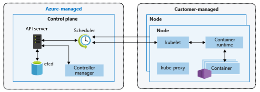
At a high level:
- Azure manages the Kubernetes control plane (API server, scheduler, etcd)
- You manage the worker nodes (VM size, scaling rules, node pools)
- Kubernetes manages your containers and workloads
This division of responsibility is deliberate. It allows teams to focus on applications and platforms rather than infrastructure mechanics.
You still get:
- Native Kubernetes APIs
- Open‑source tooling (kubectl, Helm, GitOps)
- Portability across environments
But without needing to design, secure, patch, and operate Kubernetes from scratch.
Why Should You Care About AKS?
The short answer:
AKS enables teams to build scalable platforms without becoming Kubernetes operators.
The longer answer depends on the problems you’re solving.
AKS becomes compelling when:
- You’re building microservices‑based or distributed applications
- You need horizontal scaling driven by demand
- You want rolling updates and self‑healing workloads
- You’re standardising on containers across teams
- You need deep integration with Azure networking, identity, and security
Compared to running containers directly on virtual machines, AKS introduces:
- Declarative configuration
- Built‑in orchestration
- Fine‑grained resource management
- A mature ecosystem of tools and patterns
However, this series is not about adopting AKS blindly. Understanding why AKS exists—and when it’s appropriate—is essential before we design anything production‑ready.
AKS vs Azure PaaS Services: Choosing the Right Abstraction
Another common—and more nuanced—question is:
“Why use AKS at all when Azure already has PaaS services like App Service or Azure Container Apps?”
This is an important decision point, and one that shows up frequently in the Azure Architecture Center.
Azure PaaS Services
Azure PaaS offerings such as App Service, Azure Functions, and Azure Container Apps work well when:
- You want minimal infrastructure management responsibility
- Your application fits well within opinionated hosting models
- Scaling and availability can be largely abstracted away
- You’re optimising for developer velocity over platform control
They provide:
- Very low operational overhead – the service is an “out of the box” offering where developers can get started immediately.
- Built-in scaling and availability – scaling comes as part of the service based on demand, and can be configured based on predicted loads.
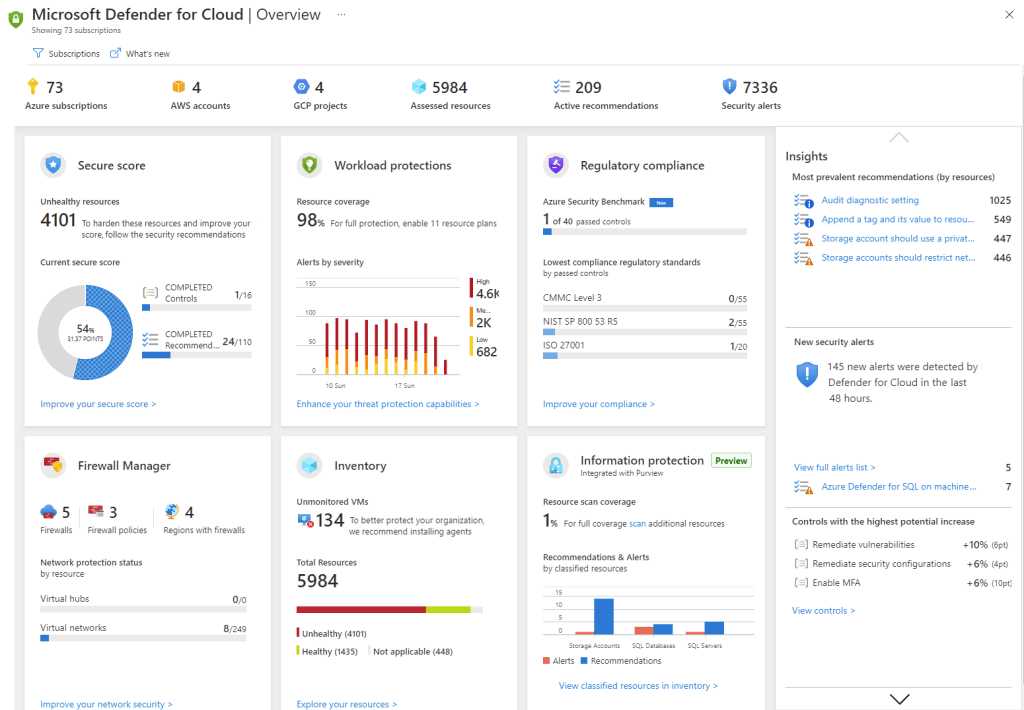
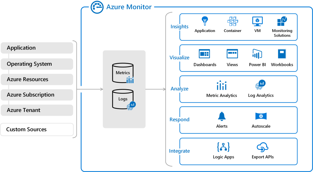
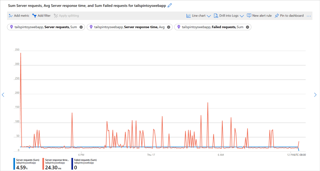
- Tight integration with Azure services – integration with tools such as Azure Monitor and Application Insights for monitoring, Defender for Security monitoring and alerting, and Entra for Identity.
For many workloads, this is exactly the right choice.
AKS
AKS becomes the right abstraction when:
- You need deep control over networking, runtime, and scheduling
- You’re running complex, multi-service architectures
- You require custom security, compliance, or isolation models
- You’re building a shared internal platform rather than a single application
AKS sits between IaaS and fully managed PaaS:
Azure PaaS abstracts the platform for you. AKS lets you build the platform yourself—safely.
This balance of control and abstraction is what makes AKS suitable for production platforms at scale.
Exploring AKS in the Azure Portal
Before designing anything that could be considered “production‑ready”, it’s important to understand what Azure exposes out of the box – so lets spin up an AKS instance using the Azure Portal.
Step 1: Create an AKS Cluster
- Sign in to the Azure Portal
- In the search bar at the top, Search for Kubernetes Service
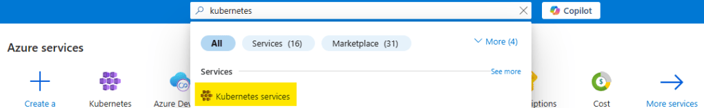
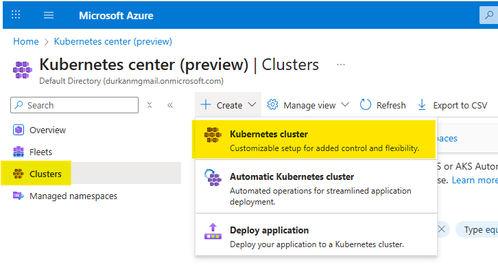
- When you get to the “Kubernetes center page”, click on “Clusters” on the left menu (it should bring you here automatically). Select Create, and select “Kubernetes cluster”. Note that there are also options for “Automatic Kubernetes cluster” and “Deploy application” – we’ll address those in a later post.
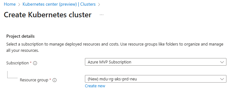
- Choose your Subscription and Resource Group
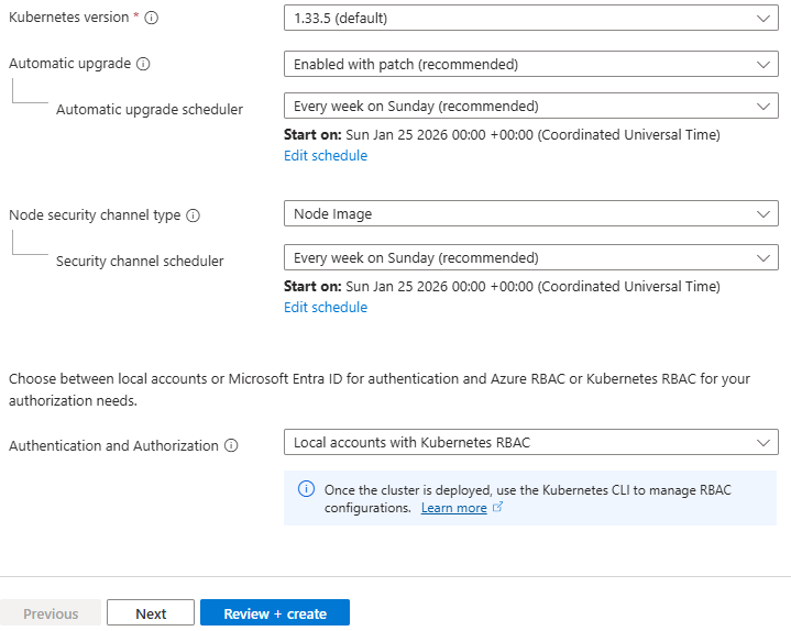
- Enter a Cluster preset configuration, Cluster name and select a Region. You can choose from four different preset configurations which have clear explanations based on your requirements
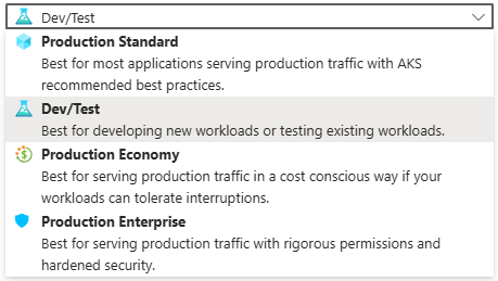
- I’ve gone for Dev/Test for the purposes of spinning up this demo cluster.
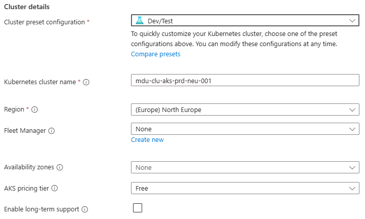
- Leave all other options as default for now and click “Next” – we’ll revisit these in detail in later posts.
Step 2: Configure the Node Pool
- Under Node pools, there is an agentpool automatically added for us. You can change this if needed to select a different VM size, and set a low min/max node count
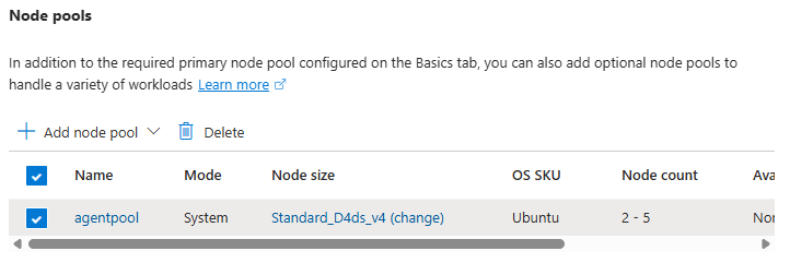
This is your first exposure to separating capacity management from application deployment.
Step 3: Networking
Under Networking, you will see options for Private/Public Access, and also for Container Networking. This is an important chopice as there are 2 clear options:
- Azure CNI Overlay – Pods get IPs from a private CIDR address space that is separate from the node VNet.
- Azure CNI Node Subnet – Pods get IPs directly from the same VNet subnet as the nodes.
You also have the option to integrate this into your own VNet which you can specify during the cluster creation process.
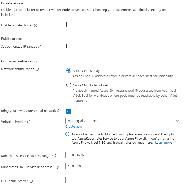
Again, we’ll talk more about these options in a later post, but its important to understand the distinction between the two.
Step 4: Review and Create
Select Review + Create – note at this point I have not selected any monitoring, security or integration with an Azure Container Registry and am just taking the defaults. Again (you’re probably bored of reading this….), we’ll deal with these in a later post dedicated to each topic.
Once deployed, explore:
- Node pools
- Workloads
- Services and ingresses
- Cluster configuration
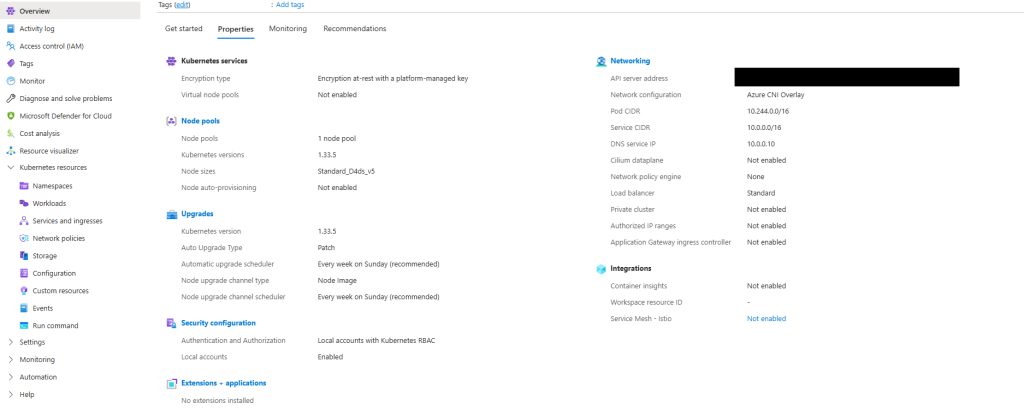
Notice how much complexity is hidden – if you scroll back up to the “Azure-managed v Customer-managed” diagram, you have responsibility for managing:
- Cluster nodes
- Networking
- Workloads
- Storage
Even though Azure abstracts away responsibility for things like key-value store, scheduler, controller and management of the cluster API, a large amount of responsibility still remains.
What Comes Next in the Series
This post sets the foundation for what AKS is and how it looks out of the box using a standard deployment with the “defaults”.
Over the course of the series, we’ll move through the various concepts which will help to inform us as we move towards making design decisions for production workloads:
- Kubernetes Architecture Fundamentals (control plane, node pools, and cluster design), and how they look in AKS
- Networking for Production AKS (VNets, CNI, ingress, and traffic flow)
- Identity, Security, and Access Control
- Scaling, Reliability, and Resilience
- Cost Optimisation and Governance
- Monitoring, Alerting and Visualizations
- Alignment with the Azure Well Architected Framework
- And lots more ……
See you on the next post!